The Two-Envelope Fallacy- A probability paradox

Introduction

A paradox is a statement that is self-contradictory in nature but might seem to be correct or true at first. Paradoxes may also arise in probability. This happens because of the ambiguous nature in which the policy has been framed. Such a situation opens the door to numerous interpretations of the same problem which might seem paradoxical.

There are many paradoxes in probability theory that include the Newcomb’s paradox, the betting crowd paradox, the open box problem, the doomsday argument, the Hadron collider card game, Berkson’s paradox, sleeping beauty problem, two envelopes problem, Bertrand’s box paradox, the Monty Hall problem, the two boys problem or the boy-girl problem, three prisoner’s problem, etc.

Understanding the problem and the Paradox

Let us understand the two envelopes problem in detail and let us try to solve it. The two envelopes problem is one of the most popular problems or paradoxes from probability theory. According to the two envelopes problem, a person is given the liberty of choosing an envelope from the two given envelopes. It is given that one envelope contains double the money than in the other envelope. The person who is asked to pick one envelope is unaware of the amount of the money contained in the closed envelopes. But before choosing an envelope, the person is again provided with an opportunity or an option to reconsider his decision of which envelope to choose. Here comes the dilemma as a person may not be sure if he must consider his first choice or should he alter it. Let us consider this situation using variables to enhance our understanding. Let us assume that one envelope contains ‘a’ amount of rupees. Therefore, according to our assumption, the other envelope will contain either ‘2a’ or ‘a/2’ amount of money as we started with the assumption that one envelope contains double the amount of money than in the other. The probability that the chosen envelope contains ‘a/2’ amount of money is ½ and likewise is the probability for the chosen envelope to contain ‘2a’ amount of money. Therefore, the average expected amount of money the person will get for switching will be ½ (2a + a/2) which will be equal to 5a/4. Hence, the amount of money obtained is 5a/4 which is obviously larger than ‘a’ amount of money. Going by this philosophy or belief, the person must swap the envelopes before picking one. But here is where the confusing part starts as according to the belief stated above, the person must swap the envelopes again before choosing which one to select and open. Going by the same argument, the person may be tempted to swap the envelope a third time and so on. Going by this thought process, a person will get caught in an infinite loop of swapping and may end up getting no money at all.

What makes the Two-Envelop Paradox counterintuitive?

Where the fallacy comes in our reasoning? Where we go wrong? Well, the answer is that the belief or the philosophy as discussed above makes this condition counterintuitive because an ordinary individual will believe in swapping again and again as according to their belief, they must get ‘5a/4’ amount of money which is clearly higher than ‘a’ and so on and so forth. Now, this is the correct time for us to try and explore the possible solutions to this fallacy.

Possible solutions to the Paradox

                                    

                                            

In order to simplify the issue, let us consider that the envelope that the mentioned person selected at first was ‘X’ and the other one was ‘Y’. Now, let us assume that the ‘X’ letter contained ‘a’ amount of money. As we are unaware of the money in envelope ‘X’ as we haven’t the envelope, ‘a’ won’t be a fixed amount. It would rather be a random variable. Hence, it can take two values, either the lesser amount of money or the larger amount of money which is hidden in the two envelopes. Let’s assume ‘2b’ to be the larger amount and ‘b’ to be the lesser amount of money. As the person picks up the ‘X’ envelope randomly, there is a fifty-fifty chance that ‘X’ contains either of the two amounts. This implies that the expected money in envelope ‘X’ is E(X) = ½ (b + 2b) = 3b/2. It has been mentioned above that the amount of money in envelope ‘Y’ is E(Y) = ½ (2a + a/2).

As ‘a’ isn’t a fixed which was mentioned above; therefore, one of the two values can be taken. In the case that the ‘Y’ envelope contained ‘2a’, envelope ‘X’ would contain the smaller amount; therefore, a = 2b. Hence, in the equation E(Y) = ½ (2a + a/2), the first ‘a’ stands for ‘b’ and the second ‘a’ stands for ‘2b’. In reality, the two ‘a’ which has been used are unlike each other and cannot be simply added.

Similarly, E(Y) = ½ (2b + b).

Therefore, E(X) = E(Y). Hence, there is no added benefit or incentive in switching the envelopes and hence the paradox is solved and is no longer a paradox. Now let us try and examine what mistakes we all were making initially taking clues from the probability theory. 

Correcting the misapplication of the conditional probability theory

In our initial workings, we had assumed that the second choice is independent of the first choice, but in reality, this is not the case and the paradox arises because of this.

If the second envelope chosen by the player contains less money than the first it is guaranteed that the person would be swapping it for the one containing double the money (say ‘2a’ rupees) at a loss of ‘a’ rupee.

Similarly, if the second envelope chosen by the person contains more money than the first, it is guaranteed to be swapped with the one containing half the amount (say ‘a’ rupee) at a gain of ‘a’ amount of rupee.

Mathematically the expectation value of the second envelope will be represented as,

 E (Second envelope = Y)  = E (Y/ X<Y)P(X<Y) + E(Y/X>Y) P(X>Y)

Taking a numerical example to make understanding clearer.

Let’s consider that either of envelope X or Y contains 100 rupees and the other contains 200 rupees. We don’t know exactly which one contains how much amount of money. Therefore, if X contains 100 rupees Y necessarily contains 200 rupees, not 50 rupees.

Now the expected value of the second envelope can be written as-

Probability(X=100) *100 + probability of (X=200) *200

OR expectation value= ½ * 100+ ½ * 200 = 150

Hence the expectation value is exactly in the middle of the range between the values 100 and 200 as you would expect it to be intuitively. Hence you should not bother swapping.

We can understand it more intuitively by taking the total amount of money involved to be 300 rupees regardless of which envelope was chosen first. But we can say for sure that the larger envelope contains 200 rupees [2(Total)/3] and the smaller envelope contains 100 rupees.

Hence the expected return from switching is equal to ½ (200-100) + ½ (100-200), making it equal to zero. Therefore, there is no advantage or disadvantage in switching the envelopes which is exactly as expected. 

Other Strategies to Solve the Two-Envelope Paradox

                                     

                                       

Randomized switching

The key to the problem occurs when the contestant opens one of the envelopes, after this information is broken out then these envelopes are not identical anymore. Researchers use the ‘cover strategy’ to explain the phenomenon which proves the players’ chance of choosing the envelope with the greater amount say 2a if played repeatedly.

The idea here is that the player would continue to switch keeping in mind the money in the first envelope. This means that a lesser amount of random switches will lead to a larger amount even though he does not know how high or low the amount is distributed among the envelopes. This cover strategy report proved that after 20000 simulations, people who followed the cover strategy had an increase in their payoff than other players who just did simple switching.

The scientists clarified that the procedure rises up out of late advances in two-state exchanging marvels that are rising in the fields of material science, designing, and financial matters. It is this thought which is behind the rule of the notable 'Parrondo's oddity, which shows that you can blend two losing games but then win.

 This answer for the two-envelope issue is a forward leap in the field of Parrondo's mystery." between two insecure states can bring about a steady condition. 

As D.Abbott stated that a Brownian ratchet is a physical gadget that can arrange arbitrary particles to stream a specific way. He said,

"The stunt with a Brownian ratchet is that again it utilizes breaking balance, It is this thought behind the rule of the notable 'Parrondo's oddity,' which shows that you can blend two losing games but then win. This answer for the two-envelope issue is a forward leap in the field of Parrondo's mystery."

Winning while losing (Strategy to solve the new envelope problem)

Although a player can utilize the arbitrary changing methodology to win cash while having earlier information on the measurable circulation of the envelopes' qualities, the huge point is that this information isn't vital. It is astounding that the examination shows that one can generally improve their benefit utilizing Cover's technique with the obliviousness of 'as far as possible' (the most noteworthy estimation of cash permitted) and of the factual conveyance the numbers comply. Also, the explanation it is of significance is that engineers regularly need to consider what are called 'daze advancement' issues. Thus the answer may invigorate a new workaround there.

Another kind of improvement technique that imparts likenesses to the two-envelope issue is monetary putting resources into the securities exchange. For example, in "instability siphoning," exchanging between helpless ventures can bring about winning an exponentially expanding measure of cash. 

Instability siphoning is a 'toy model' that one cannot utilize precisely in its current structure on the financial exchange. It is a toy model that shows hidden systems that are valuable. It proposes the intensity of changing your arrangement of stocks occasionally, purchasing low, and selling high. Both the two-envelope process in addition to unpredictability siphoning show up firmly identified with Brownian ratchet marvels. The two of them misuse the communication of asymmetry with irregularity.

This understanding likewise carries with it various open inquiries. For instance, when playing a group of games, a player could adjust the subtleties of the technique by ceaselessly refreshing the evaluated circulation from which the envelopes' qualities are picked. Likewise, since the system identifies with two-state exchanging in different fields, maybe it might be conceivable to clarify every one of these wonders with a typical scientific structure.

Conclusion

Well, quite frankly we managed to cover the most basic, simple, and lucid explanation of the paradox which is otherwise quite complex and greatly discussed and deliberated upon in academia. There are numerous explanations and possible solutions to this celebrated paradox of the probability theory called 'The- two Envelope Fallacy'. 

Our discussion also persuaded us to realize the importance of probability theory concepts such as Bayes' Theorem, Conditional Probability, Prior and Posterior concepts of the probability theory. If anyone of you got motivated and the inner curiosity got ignited, please read more on these probability paradoxes. As it is evident from our discussion, there are numerous applications of these paradoxes, so it becomes very important to know and enjoy these beautiful and tricky concepts. 💡

Authors-

Aditya Nariyal 1933406

Aditya Pratap Verma 1933407

G. M. Shibi 1933416

John Joseph 1933420

References

Agnew, R. (2004). On the two box paradox . Math Magazine, 302- 308.

F. Jackson, P. M. (1994). The two Envelopes paradox. 43-45.

M. Clark, N. S. (2000). The two envelope paradox. 415- 442.

Paradox. (n.d.). Retrieved from https://www.merriam-webster.com/dictionary/paradox

Probability, P. i. (n.d.). Retrieved from https://brilliant.org/wiki/paradoxes-in-probability/

solved, T. t. (2018, 06 22). Retrieved from https://plus.maths.org/content/two-envelopes-problem- resolution

Looking Glass Universe. (2017, January 29). Resolution of the two envelope fallacy. [Video file]. Retrieved from https://www.youtube.com/watch?v=FXNKWxwcX9U.

Impact of Monetary Policy In Resolving The Great Recession In USA

Abstract

This essay provides an analytical description of the great recession of 2007-2009. With an emphasis on the USA, this paper tries to explore the underlying causes of the recession and the consequences of the financial crisis and the credit crunch. This paper also deals with the policy actions taken to mitigate the effects by the US government and the Fed. Monetary policy measures were considered in detail and last but not least IS-LM framework was used as supporting evidence to discuss the effectiveness of the monetary policies. The paper is also backed up by considerable empirical evidence gathered from research papers and free government/world bank databases. 

Keywords: Crisis, IS-LM framework, Credit Crunch, Recession, Monetary policy, fiscal stimulus, CDO, mortgage.

Introduction and Overview 

After the boom years of 2002-07 the world economy especially the United States, the United Kingdom, and the rest of European economies, faced a catastrophic turnaround and they faced a recession during the years 2007-09 as 2009 became the first year since the second world war when the world was in recession (Islam, 2010).

The effect of the global financial crisis or the great recession whatever we may call it lead towards the huge economic downturn from the last quarter of 2007 to the third quarter of 2009 in the United States (Christiano, 2017). 

The economic crisis which had its impact on the activities of largely every country and region emanated from the credit markets in the USA and other developed countries. As a result of it, the atmosphere of easy credit conditions transformed into a situation of ‘credit crunch’ (situation of tight credit conditions), and in some cases, it had also lead to dysfunctional markets.

The global financial crisis of 2008 lead towards the decline of confidence in individual consumers and business entities leading to a significant impact on the global activity. There was already this large run-up in housing construction and dwelling prices in response to the rising policy rates during the mid of the year 2006 which had a dampening impact on the economy of the United States. In the background of extreme uncertainty, the households reduced their consumption and the demand for manufactured goods. All of these events lead towards an extraordinary fall in industrial production worldwide by the end of the year 2008 and the GDP of the US along with other major economies contracted (Edey, 2009).

Causes 

To overcome the recession in 2001, US monetary authorities kept on reducing the policy rates to unusually low levels. This helped to overcome the 2001 recession and ensured that it is short-lived but the resulting boom in the economy was largely due to the debt-financed consumption which had managed to increase the aggregate demand globally set the stage for the impending recession of 2009-09 (Islam, 2010).

Astley et al (2009) as cited in Islam (2010), held the US housing market as the force that triggered the Great Recession. The delinquency of credits which had started during the year 2006 gained momentum when the US Federal Reserve started to increase the interest rates. With larger and larger delinquencies and the rise of bad loans, many mortgage lenders declared bankruptcy and failed.  The sub-prime market uncoiled. One of the most serious implications of the complex financial products such as CDOs and credit default swaps, many financial institutions did not have any idea about the size of losses. As a result, the institutions started hoarding liquidity leading towards the freezing of the market for asset-backed commercial papers. The resultant credit crunch resulted in the increased perceptions of risk and shortfall in lending. However, the collapse of the investment bank Lehman Brothers led to a fall in the financial system in September 2008.

Due to the expected increase in the interest rate, customers felt the inability to repay the loans and in order to get some additional gain decided to sell their house. Banks in order to cover the loan risks also increased the interest rates from 3% to 5%. And when the borrowers tried to sell their houses, the increased interest rates had caused the scarcity of potential customers and since they did not find the buyers the housing prices started to fall, and bubble burst. This lead to the borrowers defaulting on the loans and banks faced to empty houses. All these chronologies of events started the chain reaction of bank failures one after another and the global recession started (Azar; Mansouri, 2011).

Many economists as mentioned by Christiano (2017) believe that the financial crisis was caused by a mix of declining house prices, shadow banking system, heavy investment of the financial system in house-related assets coupled with the interlinking of factors such as loose monetary policy, global imbalances, lax financial regulation along with the misperception of risks (Islam, 2010) lead to this financial crisis of 2008.

All these factors also led to a reduction in household wealth following the credit crunch and declining purchase of houses with a fall in the housing prices. Households cut back on spending. This caused the sales to decline substantially and the firms pull back on investment and hiring. All these factors reinforced one another and horned the economy into the tailspin of recession (Christiano, 2017).

Consequences

Of all the other consequences, the great recession also had a disproportionately large impact on the discipline of macroeconomics, and economists were forced to reconsider the discarded theories such as the IS-LM framework, etc. The damage which the national economies had top face is yet to recover.  There was a severe impact on macroeconomic variables such as consumption, employment, investment, output, etc. The drop in the magnitude of these variables was larger than the average of all the recessions since 1945. The decline in Employment, for example, was 6.7% and for consumption and output, it was 5.4% and 7.2% respectively (Christiano, 2017).

A global job crisis also emerged from the global financial crisis as the tightening credit conditions damaged the real economy and the trades collapsed. Unemployment increased like anything and millions were impoverished. The United States economy as the USA was at the epicenter of the crisis was hit severely. The US economy after falling into the recession shrunk by 2.7% by the year 2009 and largely these repercussions were the results of the financial crisis and the credit crunch. In the USA due to the fall in prices, there was an increase in the real wage. The falling prices also led to an increase in real hourly earnings. Interestingly the great recession had contributed to the correction of the previously deteriorating real hourly wages which were fueled by the rising inflation and constant nominal wages before the financial crisis of 2008-09 (Islam, 2010).

An average household in the USA lost nearly $5,800 of income as a consequence of the lowered economic growth. On the other hand, the Fed spent $2,050 on average, for each household to alleviate the effects of the financial crisis. The total loss summed up to about $100,000 per household due to the combined effects of the fall in house prices and the prices of the stock during the periods of the great recession between July 2008 to March 2009 (Swagel, n.d.).

Policy Response

The policy response to the crisis incurred gigantic costs to the US government as the public debt was already high due to the low levels of revenues and high levels of the spending to mitigate the impacts of the crisis (Swagel, n.d.).

In the United States, noticeable measures were taken to remove the bad assets from the balance sheet of affected financial corporations and to purchase the long term securities for supporting the mortgage and the private credit markets (Edley, 2009).

We can therefore conclusively group the US policy response into two broad categories:

1. Measures to target the immediate issues of reconstructing the damaged credit markets and regain the demand and other economic activities.

2. Measures directed to reduce the risk of occurrence of a similar crisis in the future.

According to the works of Azar and Mansouri (2011), the governments tried to inject massive amounts of credit into the financial markets. They also went for nationalizing the banks, lowered the interest rates, and increased discretionary spending by the means of fiscal stimulus packages. Thus, we can categories the policy response in the view of the great recession in the following categories: 

1. For keeping the credit flowing the devised bailouts to inject money into the financial systems.

2. To deal with the credit crunch they slashed down the interest rates. Thus stimulating the borrowings and investment.

3.  There was a fiscal stimulus to increase aggregate demand.

Monetary Policy Response And Its Impact

Initially, in the wake of the housing market collapse in 2007, the Federal Reserve System continued to increase the supply of money and kept on lowering the interest rate. This managed to keep the economy afloat until the end of the year 2008. Then arrived the major problem that the interest rates were already reduced to zero and the collapse of the US housing market had caused a serious negative impact on the financial system. And since the money supply could not have been increased by way of reducing the interest rates, various monetary and fiscal actions were taken. The monetary policy actions taken to stimulate the expenditure can be discussed as follows (Sims, 2003)

1. Quantitative easing- Longer maturity rates, priced according to the safer longer terms assets (private sector debt with longer maturities, treasury bills, and bonds) such as mortgages are relevant for the firms and the consumers. And normally the monetary authorities try to affect the short term interest rates which then through a standard term structure manages to affect (lower) the longer rates. By this policy of quantitative easing, the Fed bought the longer-term assets as an attempt to directly lowering the longer-term interest rates.

2. Operation Twist- This was one of the non- standard policy of the Fed, where in order to lower the long rates, the central bank bought the bonds of longer maturity and sold the bonds of shorter maturity.

3. Forward Guidance- Fed, announced explicitly its intentions regarding the promise of lower short interest rates in the future in order to reduce the longer maturity rates in the present.

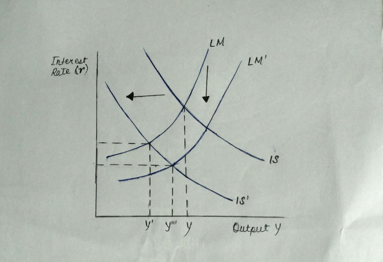
The simple understanding of these policies is that they are intended to avoid the deflation and deflationary expectations trap. The three policy majors signaled implicitly higher future inflation levels. The Fed effectively promised to bring in future expansionary monetary policy trying to raise the inflation levels. Thus, the current expected levels of inflation may also rise if people anticipate this future expansionary monetary policy. And this can stimulate investment and consumption levels provided that the nominal interest rates are already close to zero. This can be depicted by a downward/rightward shift of the LM curve as we will see next.

Now let us look at the plot of real GDP per capita of the US and we can comment on the effectiveness of the policy actions.

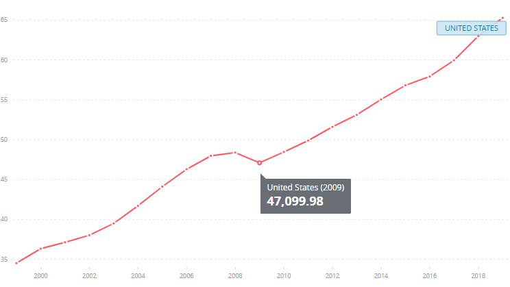
Source: The World Bank Data. Retrieved from https://data.worldbank.org/indicator/NY.GDP.PCAP.CD?end=2019&locations=US&start=1999

We can also analyze the data for consumption expenditure over the periods of the great recession and observe the changes in them to comment on the effectiveness of the policy decisions.

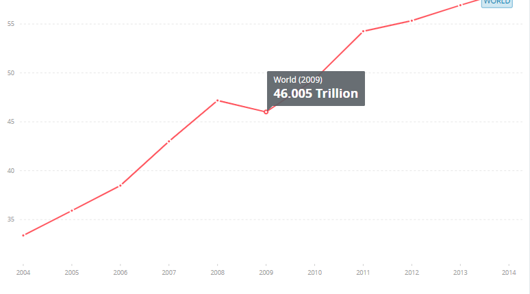
Source: The World Bank Data. Retrieved from 

https://data.worldbank.org/indicator/NE.CON.TOTL.CD?end=2014&start=2004

IS-LM Framework As Supporting Evidence 

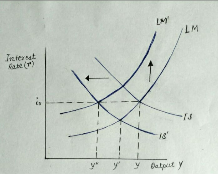
The great recession can be characterized by the negative shock to the demand for goods. This is going hand in hand with the traditional macroeconomic model captured by Hicks and Hansen in their IS-LM model (Christiano, 2017). Thus we can use this model to explore the underlying conditions about the US economy and evaluate the policy responses.

According to the works of Swain (2009) as cited in Azar and Mansouri (2011), due to the fall in personal consumption in the US, the IS curve shifted leftward. This led to the decline of the output as shown in the figure below to Y’. In order to maintain the target interest rates, there was an upward shift of the LM curve decreasing the output further to y”.

Now the Fed cut and dramatically reduced the policy interest rates. This increased the liquidity in the cash market leading towards a downward shift of the LM curve. This will offset the effect created by the leftward shift of the IS curve, attempting to maintain the output levels to y’” in the short run as indicated by the graph below. The real interest rate declines with the consumption and investment both increasing.

Conclusion

Despite all the measures the US economy took over five years to return to the 2007 level of output per capita. Empirical evidence (Christiano, 2017) suggests that the United States is still below the trend growth in 2007 by about 10%. The work also highlights that the need of the hour is to try and reduce the onset and severity of any such future crisis and global recessions.

The great recession also showed us the relevance of developing new economic theories, especially in the financial sector. Study and research in the field of international finance and economics are also very important as when a great economy like the USA faces a crisis, it becomes the global crisis.

References

Edey, M. (2009, September). The Global Financial Crisis and its Effects. Retrieved August 02, 2020, from https://onlinelibrary.wiley.com/doi/epdf/10.1111/j.1759-3441.2009.00032.x

Golmohammadpoor Azar, K. (1970, January 01). 2008 Economic Crisis Analysis: The Macroeconomic Approach. Retrieved August 02, 2020, from https://www.econstor.eu/handle/10419/49648

The Great Recession: A Macroeconomic Earthquake. (n.d.). Retrieved August 02, 2020, from https://www.minneapolisfed.org/article/2017/the-great-recession-a-macroeconomic-earthquake

Sims, E. (2013). Intermediate Macroeconomics: Great Recession. Retrieved from https://www3.nd.edu/~esims1/great_recession_fall_2013.pdf

Swagel, P. (n.d.). The Cost of the Financial Crisis: The Impact of the September 2008 Economic Collapse. Retrieved from https://www.pewtrusts.org/-/media/assets/2010/04/28/costofthecrisisfinal.pdf

Verick, S., & Islam, I. (2010, May). The Great Recession of 2008-2009: Causes, Consequences and Policy Responses. Retrieved from http://ftp.iza.org/dp4934.pdf

Behavioral Economics and Human Decision Making

                                      

In our day to day life, we make numerous decisions  about different things. These include our political decisions, personal decisions and financial decisions. Have you ever wondered what guides our decision making process and choices that we make? Well, “Behavioral Economics” is the discipline of study which tries to find out the answer to the above question. It also tries to explain what happens after the decision is made, as well as how present decisions impact future behavior and decision making.

The decision making process also depends upon the decision being made and there can be several factors which influence our decision making. To name a few, factors like past experience, cognitive biases, age and individual differences, belief in personal relevance, etc. influence the choices we make. To be able to understand what decisions are made, understanding of these factors is very important.

Human psychology and perception plays a dominant role in deciding how human beings make decisions. Perception can be defined as a process by which individuals organize and interpret their sensory impressions in order to give meaning to their environment. It becomes so important as people's behavior depends more on their perception of reality than the reality itself. Factors such as personal attitudes, motives, interests, experiences and expectations along with the time, work setting and social situation influence the perception of an individual. Why students strive so hard to clear the UPSC Civil Services Exams in India- maybe because of the perception that an IAS or IPS officer gets huge prestige besides having the vast powers of the public office.

Various types of errors and biases enter our decision making process when we try to take shortcuts while deciding. Let’s try to understand them. Among your friends, if you are considered to have a good sense of direction, you will hesitate to ask for help despite knowing the fact that you are lost while driving a car with your friends inside. This is known as Overconfidence Bias where we tend to be overly optimistic. If you are a dog lover and see a vicious dog attacking an innocent child, you tend to believe that the dog is defending itself against a menacing child. This is known as Confirmation bias which occurs when a person interprets a situation according to their own pre-existing beliefs. Few other errors/ biases in our decision making are Anchoring Bias, Availability Bias, Escalation of Commitment, etc. Hope we will discuss more about these concepts in the coming blogs.

In Behavioral Economics, we have something called the “rational choice theory” which assumes that human actors have stable preferences and engage in maximizing behavior. But this theory of rational choice has its own limitations.  It is here that we define a term called “Bounded Rationality” which states that our decisions are not always optimal. According to the works of Herbert Simon (1982) and Kahneman (2003), the term bounded rationality can be understood as restrictions to the human information processing, due to limits in knowledge (or information) and computational capacities. 

We prefer credit cards over cash transactions despite knowing the fact that it is going to cost more. Why?  The answer is quite simple and can be explained by the theory of mental accounting which says that people think of value in relative rather than absolute terms. In this situation the pain is thought to be reduced in credit card purchases, because plastic is less tangible than cash, the depletion of money is less visible and payment is deferred. We all must have experienced the moment of panic when the waiter comes to our table to take the order and we are still struggling to contemplate the appetizers on page 1 of a 10-page menu? This is referred to as Choice Overload which may lead to less satisfaction derived from our choice or reduced confidence in decision making or inhibition of any decision at all. The concept of choice overload explains well the bounded rationality of humans. Sometimes people refrain to obtain knowledge which is freely available. Research studies have shown that investors are less likely to check their portfolio online when the stock market is down than when it is up. We call this as Information avoidance in behavioral economics which goes hand in hand with our assumption of bounded rationality where people have limited ability to process the information. 

 

Now let’s see the relevance of Context in decision making which is nothing but any factor or situation which can shift the choice outcomes by altering the decision making process. It goes without saying that the situation in which the decision must be made influences the decision that is made. Here by context, we mean a combination of components like the decision need, financial aspects of the decision making, etc. Factors such as social, historic and cultural aspects of the situation also determines the context in which the decision must be made. 

Your Sunday plans might get affected when you have your exams the coming Monday, right?

Hope we have discussed some crucial aspects of the complex human decision making process. Thanks for reading. Cheers! 

Consumer Preferences and Microeconomics

We purchase various kinds of products or services. How we actually decide to buy those goods and services is an important question in microeconomics and the answer to that is known as theory of Consumer Preference. 

Consumer Choice Theory is the study of how people decide to spend their money based on their individual preferences and budget constraints. The consumer theory is not flawless as it takes into consideration a number of assumptions about human behaviour.

Economists give importance to "satisfaction" as a primary determinant of consumer preferences and a term called "utility" is defined. According to microeconomics, utility denotes the relationship between amount of goods consumed and the amount of happiness or satisfaction that a consumer gets. In other words "utility" describes the taste of consumers and it is the ability of the good to satisfy a want. 

   

To understand this concept more clearly, let's consider the case of three friends who have recently graduated their high school and are all set to go to the new cities and start their college life. And there is a laptop too in their shopping list. We know that the laptop market is mainly dominated by Windows laptops and Apple laptops called Macbooks. Armis enjoys photography and making videos and he plans to start a YouTube channel also in college. Therefore, he decided to go for Macbook over a windows os based laptop as he assigned more utility to the former than the latter. Suppose he assigned the MacBook a total utility of 10 utils and a total of 7 utils to the Windows Laptop. However, these numbers were opposite for Athos and Porthos who enjoyed playing games. They preferred windows over the Mac laptop. This approach is known as the Cardinal Utility method, where the satisfaction derived by the consumers can be quantitatively expressed. 

Now Athos ended up purchasing Dell XPS laptop while Porthos purchased Lenovo Legion laptop. They both ranked one brand over the other and there can be many reasons for it. However, this approach of not assigning any numerical units to the satisfaction derived and qualitatively measuring the utility is known as the Ordinal Utility method. This method is also known as Indifference Curve Approach.

Now let's ponder over the question- Are there any limitations to consumer preferences?  Well surely there are! Victor who used to play multiplayer games with Athos and Porthos ended up purchasing Acer Nitro 5 laptop as his finances did not allow him purchase any of those high end gaming laptops. Therefore, budget constraints, availability of the product, need of the commodity are the factors which cap consumer preferences. Thus, the consumer preferences are expected to be in accordance with few rules/ assumptions.

We can either prefer one consumption bundle over the other or be indifferent towards both the bundles. This is called the assumption of completeness. Next, we can say that consumers make consistent choices. If your girlfriend prefers Cappuccino to Espresso and Espresso to Mochaccino, you can surely order Cappuccino over Mochaccino on your date. This is the assumption of transitivity. Now we have the assumption of monotonicity i.e. consumers tend to prefer more to less. Isn't it too relatable? There are other assumptions to consumer choice theory such as the reflexivity and the convexity assumption as well.

Now let's throw some light on why the economists study Consumer Choice Theory and why is it important to to understand Consumer Preferences? The better understanding of consumer preferences has a major role to play in the relationship between the price of a good or service and the quantity demanded for a given period of time, and the shape of the overall economy because the company profits, labour market, investment, etc. depend on consumer purchases. Knowledge about Consumer Preferences also guides the firms to come up with the relevant marketing strategies to expand their reach. It is also the key to profit maximisation strategies of the firms.